In Australia, retirement funds are known as superannuation or Super for short. During your working life, you and your employer make contributions into a fund, generally of your choice.
Around a million working Australians cannot choose their fund because of enterprise bargaining arrangements or workplace determination.[Final Report] For the remaining ~14 million, we can jump ship and are free to move to the best fund available with the lowest fees.
2021 Update: The ATO have launched the YourSuper comparison comparison site https://www.ato.gov.au/YourSuper-Comparison-Tool/
According to the report, about 40% of Aussies have multiple accounts, which increases your fees! At one point I had over 3 accounts, as I moved companies I just ticked the default fund provided at each location.
There are 3 types of Super:
- self-managed superannuation trusts (SMSFs) (regulated by the ATO),
- exempt public sector superannuation schemes (regulated by Commonwealth, state or territory legislation)
- and APRA-regulated funds regulated by the Australian Prudential Regulation Authority (APRA) under the Superannuation Industry (Supervision) Act
The APRA funds, and their MySuper products are what I will cover, as it contains the bulk of the funds of which one can choose from.
MySuper products are Low-cost, simple superannuation products for members who make no active choice about their superannuation.[Final Report]
From the Royal Commission, the report recommended that APRA be given a new role which was more focused on member outcomes, and proposed that APRA would oversee and promote the overall efficiency and transparency of the superannuation system, to the ultimate benefit of members, i.e. Us and our money.
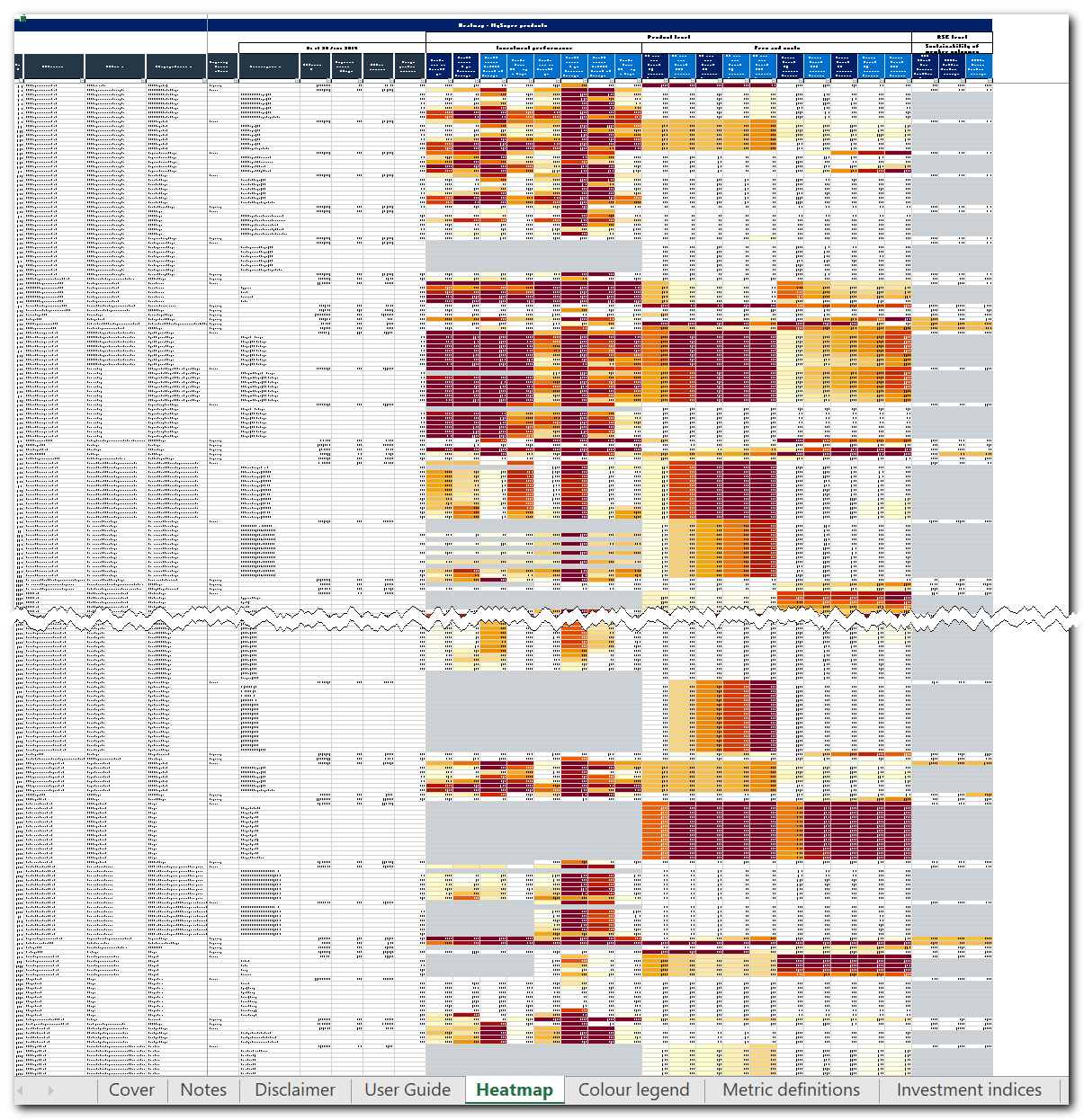
APRA came out with their MySuper Product Heatmap, which is a good start but good but is overwhelming to understand.
While APRA recognises that net return has value as a headline indicator, it is important to look separately at the drivers of net returns – namely, net investment returns and administration fees – to draw further insights.[APRA Data Insights]
What I will cover here is some slicing and dicing of APRA’s data in Python and producing some simplified heatmaps. I have included the final heatmaps at the start, then I walkthrough the steps in Python.
Performance Simplified
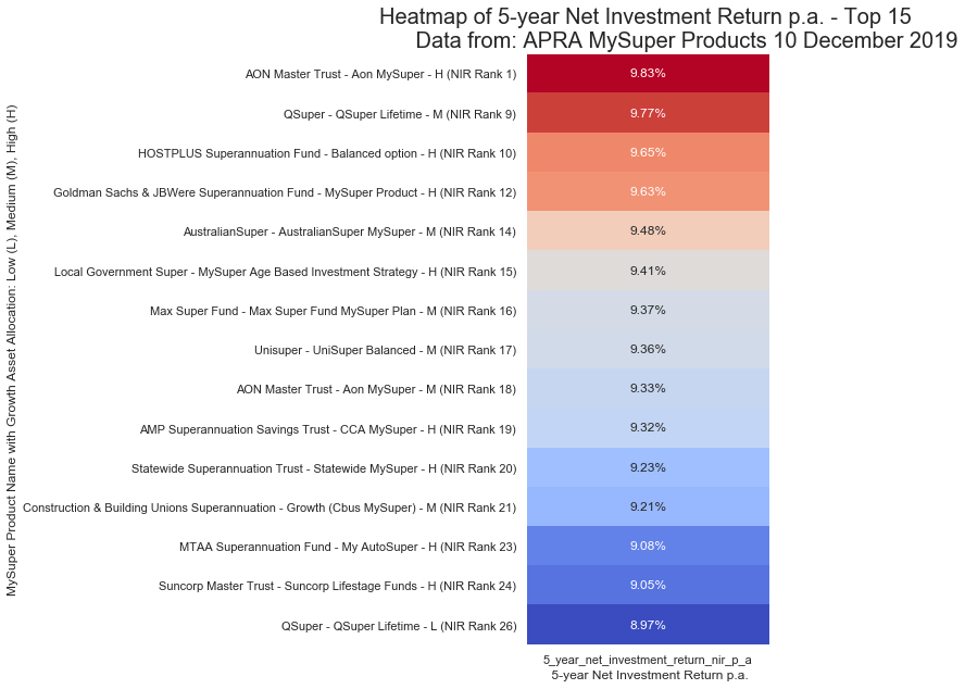
Net Investment Return – Heatmap of Top 15 Funds
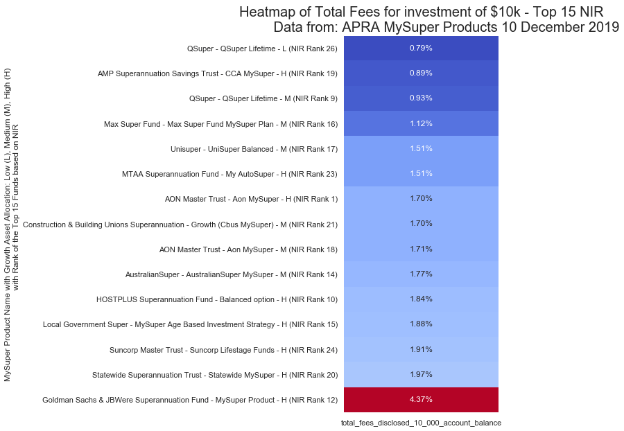
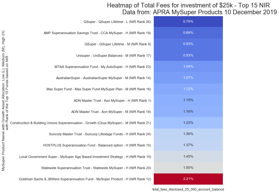
Total Fees per Investment Size – Simplified
$10,000 Investment
$25,000 Investment
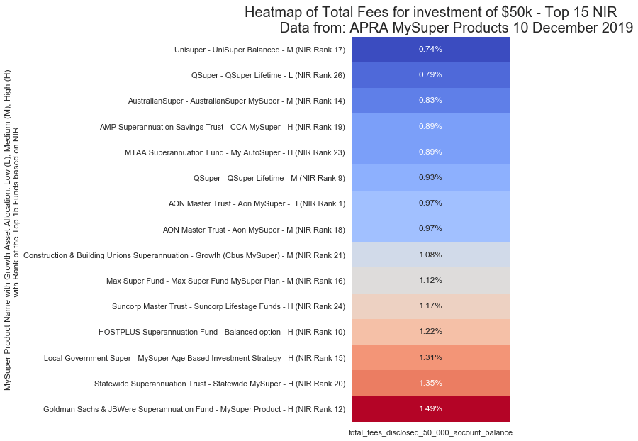
$50,000 Investment
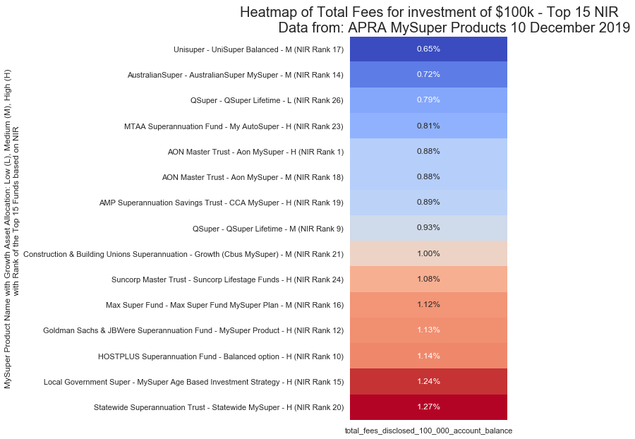
$100,000 Investment
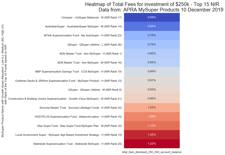
$250,000 Investment
Python Walkthrough
Read in the Data
APRA provides both a Microsoft Excel XLSX file and a comma-separated CSV file.
fp_1 = r'C:UsersbernoOneDriveLearningPythonScriptsdataMySuper Product Heatmap.csv'
skiprows_1 = 0
# Read in csv file
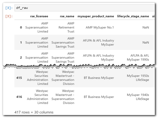
df_raw = pd.read_csv(Path(fp_1), skiprows=skiprows_1)Let’s take a quick look at the data frame to check that everything was read in correctly or not.
Next is to see all the column names and a count of missing values. I am only interested in the total fees and funds that have a 5-year net investment return.
fn_check_missing_data(df_raw)
rse_net_rollover_ratio_3_year_average                        320
rse_adjusted_total_accounts_growth_rate_3_year_average       320
single_strategy_lifecycle_indicator                          320
rse_net_assets_000                                           320
proportion_of_total_assets_in_mysuper                        320
rse_total_accounts                                           320
rse_net_cash_flow_ratio_3_year_average                       320
5_year_net_investment_return_nir_p_a                         154
5_year_nir_relative_to_simple_reference_portfolio_p_a        154
5_year_nir_relative_to_listed_saa_benchmark_portfolio_p_a    154
5_year_net_return_50_000_rep_member_p_a                      154
3_year_nir_relative_to_listed_saa_benchmark_portfolio_p_a    138
strategic_growth_asset_allocation                            138
3_year_net_investment_return_nir_p_a                         138
3_year_nir_relative_to_simple_reference_portfolio_p_a        138
3_year_net_return_50_000_rep_member_p_a                      138
lifecycle_stage_name                                          97
administration_fees_disclosed_10_000_account_balance          35
administration_fees_disclosed_25_000_account_balance          35
administration_fees_disclosed_50_000_account_balance          35
administration_fees_disclosed_100_000_account_balance         35
administration_fees_disclosed_250_000_account_balance         35
total_fees_disclosed_10_000_account_balance                   35
total_fees_disclosed_25_000_account_balance                   35
total_fees_disclosed_50_000_account_balance                   35
total_fees_disclosed_100_000_account_balance                  35
total_fees_disclosed_250_000_account_balance                  35
mysuper_product_name                                           0
rse_name                                                       0
rse_licensee                                                   0
I will now assign a new dataframe to those columns I wish to keep.
# Define columns of interest
cols_1 = ['rse_name', 'mysuper_product_name',
                   'strategic_growth_asset_allocation',
                   '5_year_net_investment_return_nir_p_a',
                    'total_fees_disclosed_10_000_account_balance',
                    'total_fees_disclosed_25_000_account_balance',
                    'total_fees_disclosed_50_000_account_balance',
                    'total_fees_disclosed_100_000_account_balance',
                    'total_fees_disclosed_250_000_account_balance']

# Assign dataframe with only columns of interest
df = df_raw.loc[:,cols_1]
Another quick review of the new dataframe.
df.info()
<class 'pandas.core.frame.DataFrame'>
RangeIndex: 417 entries, 0 to 416
Data columns (total 9 columns):
 #   Column                                        Non-Null Count  Dtype
---  ------                                        --------------  -----
 0   rse_name                                      417 non-null    object
 1   mysuper_product_name                          417 non-null    object
 2   strategic_growth_asset_allocation             279 non-null    float64
 3   5_year_net_investment_return_nir_p_a          263 non-null    float64
 4   total_fees_disclosed_10_000_account_balance   382 non-null    float64
 5   total_fees_disclosed_25_000_account_balance   382 non-null    float64
 6   total_fees_disclosed_50_000_account_balance   382 non-null    float64
 7   total_fees_disclosed_100_000_account_balance  382 non-null    float64
 8   total_fees_disclosed_250_000_account_balance  382 non-null    float64
dtypes: float64(7), object(2)
memory usage: 29.4+ KB
Of the 417 funds, there are only 263 which have reported results for at least the last 5-years, so I will drop those funds that haven’t reported.
# Drop empty rows
df.dropna(axis=0, how='any', inplace=True)
df.info()
Let’s have a quick glance over two columns to see if things make sense.
df[['5_year_net_investment_return_nir_p_a', 'total_fees_disclosed_100_000_account_balance']].describe()| 5 year NIR p.a. | Total fees 100k balance | |
|---|---|---|
| count | 263.0000 | 263.0000 |
| mean | 0.0729 | 0.0101 |
| std | 0.0152 | 0.0023 |
| min | 0.0375 | 0.0050 |
| 25% | 0.0624 | 0.0088 |
| 50% | 0.0768 | 0.0098 |
| 75% | 0.0834 | 0.0113 |
| max | 0.0983 | 0.0182 |
The 5-year return p.a. ranges from 3.75% to 9.83%. We want to be near the top end of this stat. The total fees on a $100k balance range from 0.5% to an eye-watering 1.82% (that is a whopping +300% difference). We want to be near the bottom end of this stat!
All figures appear reasonable, no negative percentages (which could happen in the returns but never in the fees)
File Specific Functions
Refer to the code on GitHub. I don’t think it warrants dumping the slew of code here.
Cleaning
The original dataset was clean, so no cleaning required. I’ve added a few columns to the dataframe for later use. I included some comments for each.
# General cleanups

# Replace a really long name
df['mysuper_product_name'] = df['mysuper_product_name'].str.replace(
    'Goldman Sachs & JBWere Superannuation Fund_MySuper Product', 'MySuper Product')

# Add a column to group the growth asset allocations into Low, Medium, High
# Change from categorical type to string for use in charts
df['growth'] = pd.qcut(df['strategic_growth_asset_allocation'], q=3,
                                             labels=['L', 'M', 'H']).astype('str')

# Assign a ranking to the 5-year NIR for later comparisons
df['5_yr_nir_ranking'] = df['5_year_net_investment_return_nir_p_a'].rank(method='min',                                        ascending=False).astype('int')

# Assign a ranking column to string type for later use in charts
df['5_yr_nir_rank_str'] = df['5_yr_nir_ranking'].astype('str')

# Add a concatenated column for use in the heatmap
df['MySuper_Details'] = df['rse_name'] + ' - ' +                                                  df['mysuper_product_name'] + ' - '
                       + df['growth'] + ' (NIR Rank ' +                                          df['5_yr_nir_rank_str'] + ')'
To get an idea of the returns distribution, the value_counts will do the trick.
# Check the breakdown of the NIR
df['5_year_net_investment_return_nir_p_a'].value_counts(normalize=True, bins=3)
(0.078, 0.0983] 0.4639
(0.0578, 0.078] 0.3460
(0.0364, 0.0578] 0.1901
Name: 5_year_net_investment_return_nir_p_a, dtype: float64About 19% has returns less than 5.8% with the remaining 81% returning over 5.8% p.a. over the past 5-years.
I set the risk tolerance (growth column) into 3 equal buckets according to their strategic growth asset allocation. We could refine this, but I think it provides a reasonable split.
Analysis
Now comes the most fun bits, seeing what we can garner from the data.
For starters, I will run some checks and comparisons with the source data material to ensure everything is jiving well.
Scatterplot – NIR vs Fees for a set Growth Allocation
APRA prepared a Data Insights file with graphs and commentary to supplement the heatmap data. On page 9 of the pdf, Figure 3 below shows a negative relationship between net returns and total fees over 5 years with an allocation to growth assets greater than 60%. Let’s see if we can create something similar.
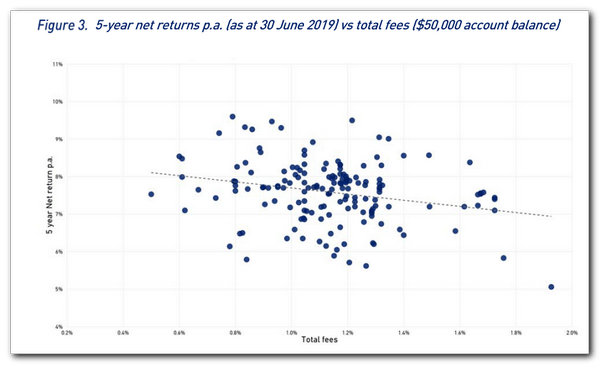
First, I will set a strategic growth asset allocation of 0.6 (60%) to match that in ARPA Figure 3. Then I will assign a dataframe based on this condition and pass it into a scatterplot with code sourced from StackOverflow how-to-overplot-a-line-on-a-scatter-plot-in-python and format-y-axis-as-percent.
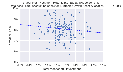
The result is like Figure 3 keeping in mind the dates of the data vary from 10 December vs. 30 June. The trend is heading downward, which goes to show that the higher the fees the lower the $ return.
Heatmap – Variable Correlations
APRA Figure 4 (not shown here) showed a weak correlation between returns versus fees (correlation was -0.1). This is a good sign, which means paying higher fees has a weak link to your expected returns, or find a low fee fund!
To see if the data has any other potential relationships (or correlations), we can either run a df.corr() or produce this cool looking half masked heatmap that I discovered by Manu Kalia.
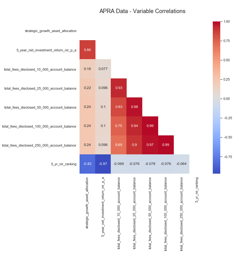
While the heatmap is aesthetically pleasing, it contains a lot of useless info for this case. So let’s just feed in the returns columns into the plotting function for evaluation.
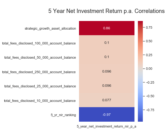
There appears to be a strong correlation between returns and the growth allocation as suspected. There is little to no correlation with returns and fees as noted by APRA.
Ranking of Top Funds Based on Return Performance
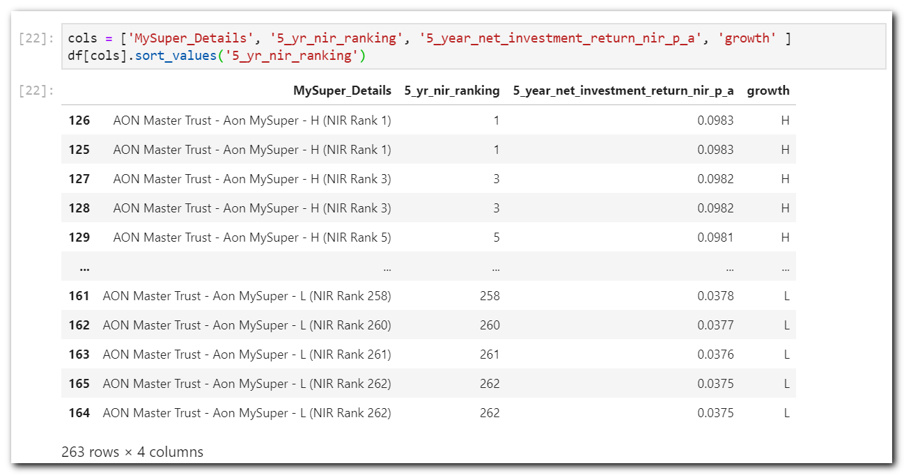
In the cleaning section, I added a column to rank the funds based on the highest 5-year return as the top-ranking using rank. But a scan through the output doesn’t tell you much as one fund is showing across the board. So grabbing the top 15 will be useless as it will only show one fund cause they provided multiple investment options with varying growth asset allocations.
Pandas ranking method ranks the records the same when their values are the same. The first two records in the table both have a rank of 1 cause their 5-year returns are the same value. Refer to the pandas docs for more details.
Getting the top 15 using nlargest again captures the same fund multiple times. What we want to achieve is a single fund per risk tolerance as defined as High, Medium, Low and output their best respective return/rating. For example, we want to get AON Mater Trust with High growth as a single line with their highest return of 9.83% then followed by QSuper with Medium growth with a return of 9.77%, and so forth.
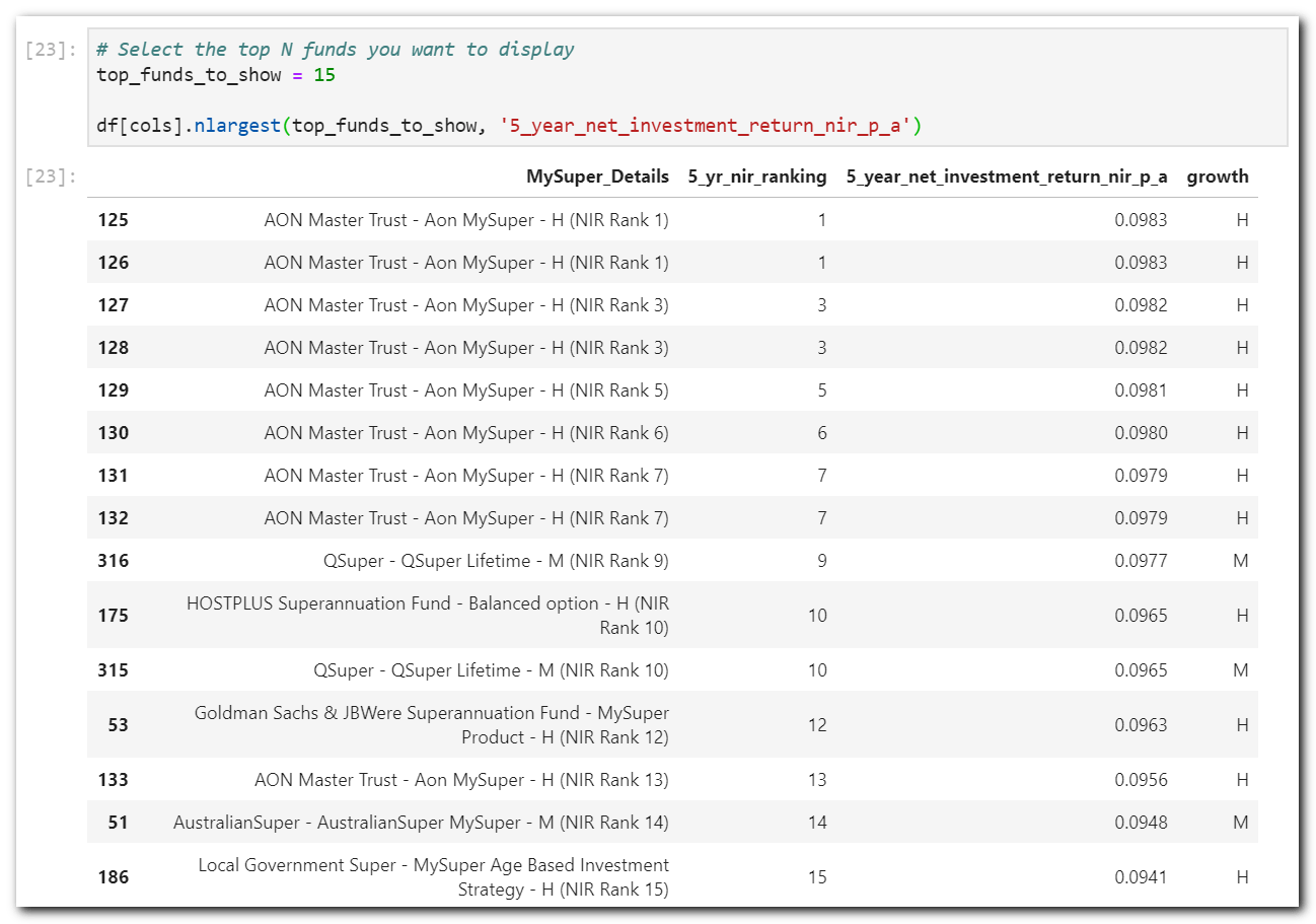
nlargest – Still not very usefulThis is a perfect candidate for pandas pivot_table. Pivot the funds to group them and extract the desired values for returns, fees and ranking.
# Assign some columns to display. Adjust to suit
cols = ['rse_name',
       '5_year_net_investment_return_nir_p_a', 'growth', '5_yr_nir_ranking', 'MySuper_Details']

# Assign a dictionary to be passed into the pivot_table aggfunc. The keys are the columns to
# aggregate and the values are the aggregate function or list of functions.


aggfunc_dict = {'5_year_net_investment_return_nir_p_a': 'max',
                # get the max return of a fund grouping

                '5_yr_nir_ranking': 'min',
                # get the min ranking as lower the number the better

                'total_fees_disclosed_10_000_account_balance': 'max',
                'total_fees_disclosed_25_000_account_balance': 'max',
                'total_fees_disclosed_50_000_account_balance': 'max',
                'total_fees_disclosed_100_000_account_balance': 'max',
                'total_fees_disclosed_250_000_account_balance': 'max',
                # get the max fees of a fund grouping

                'MySuper_Details': 'first'}
                # get the first name in the group.

# Assign some index columns to pivot on
index=['rse_name', 'mysuper_product_name', 'growth']

# Assign the column name for which to get the top N funds
performance_column = '5_year_net_investment_return_nir_p_a'

# run a pivot on the dataframe with and selecting the top N funds
pd.pivot_table(df, values=aggfunc_dict.keys(), index=index, aggfunc=aggfunc_dict
              ).nlargest(top_funds_to_show, performance_column
                        ).reset_index()[cols]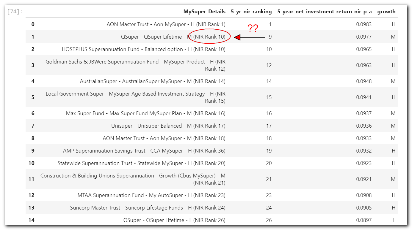
Good grief! Why are some rankings not matching? This was a bit puzzling. The purpose of the combined MySuper_Details column is the label text for the heatmap.
During pivoting the MySuper_Details function I set it to first, which seems to make sense as the first row should be towards the top.
I tried to find a clear list of functions that we can pass into the aggfunc but wasn’t able to come up with a complete list, so I had to open up the source file and have a peruse. I found the following on lines 1419 to 1424 of the groupby.py documentation: sum add np.sum prod np.prod min np.min np.max first last.
The first function sends values to numpy and returns the first value at position [0]. Based on this, I concluded that the best-ranked fund was not always at the top during the pivot operation. Sorting the dataframe in the function fixed the issue.
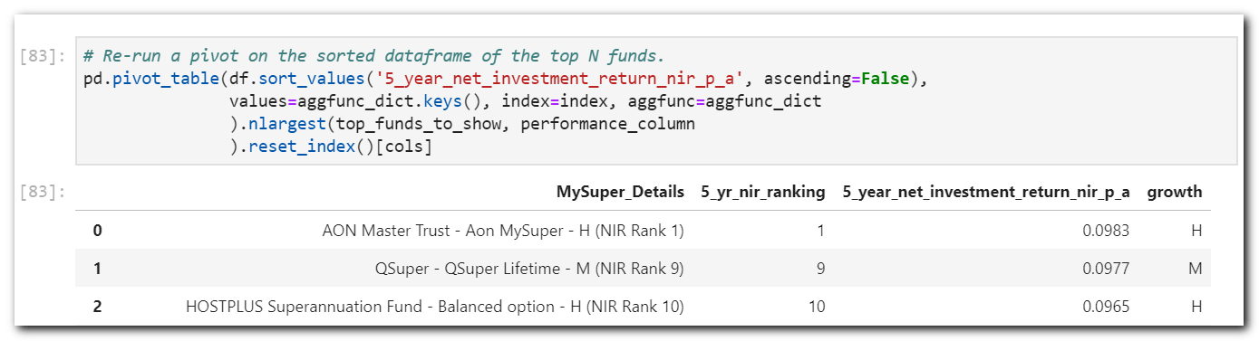
Note that I left the rankings as they appear in the original dataframe. I assume it could be reset to 1, 2, 3 etc. if that is what you desire.
As a last check, I like to confirm results from the original dataframe to ensure I hadn’t messed up my pivot tables and cleaning operations. idxmax() should do the trick.
df.loc[df['5_year_net_investment_return_nir_p_a'].idxmax(),:]rse_name AON Master Trust
mysuper_product_name Aon MySuper
strategic_growth_asset_allocation 0.8700
5_year_net_investment_return_nir_p_a 0.0983
total_fees_disclosed_10_000_account_balance 0.0170
total_fees_disclosed_25_000_account_balance 0.0115
total_fees_disclosed_50_000_account_balance 0.0097
total_fees_disclosed_100_000_account_balance 0.0087
total_fees_disclosed_250_000_account_balance 0.0082
growth H
5_yr_nir_ranking 1
5_yr_nir_rank_str 1
MySuper_Details AON Master Trust - Aon MySuper - H (NIR Rank 1)
Name: 125, dtype: objectWe have a match. All looking good, so now onto creating some simple, easy to read heatmaps to replace that convoluted one provided by APRA.
Net Investment Return – Heatmap Top N Funds
To create the heatmap of top-performing funds shown at the start of the article, I called a function by passing in the dataframe, a top number of funds to show and a filename to save the figure to the computer.
fn_pivot_table_for_heatmap(df, top_funds_to_show, 'img/apra_5_year_top_perform_heat.png')This function calls another pivot table function, which pivots the top performers as discussed above.
def fn_pivot_table_for_heatmap(df, top_funds_to_show, file=None):
    """Seaborn heatmap of top funds based on NIR
    df: dataframe
    top_funds_to_show_show: interger
    file: str value of a figure filename to save. Default is None, which doesn't save.
    """
    nir='5_year_net_investment_return_nir_p_a'

    # Get top N performers unique to each fund / risk tolerance (L, M, H)
    df_top_perform = fn_pivot_table(df, top_funds_to_show)
    df_top_perform.reset_index(inplace=True)

    # Pivot the top N performers with their details to be passed to the heatmap labels
    df_pt = df_top_perform[['MySuper_Details', nir]]

    # Set the index for use in the heatmap
    df_pt.set_index('MySuper_Details', inplace=True)

    fig, ax = plt.subplots(figsize=(4,10))

    sns.heatmap(df_pt.sort_values(nir, ascending=False), annot=True,
                cmap='coolwarm', cbar=False, fmt='.2%', ax=ax )

    plt.title(f'Heatmap of 5-year Net Investment Return p.a. - Top {top_funds_to_show} n
             Data from: APRA MySuper Products 10 December 2019',
             fontsize=20)
    plt.xlabel(f' 5-year Net Investment Return p.a.',
               fontsize=12)
    plt.ylabel('MySuper Product Name with Growth Asset Allocation: Low (L), Medium (M), High (H)',
               fontsize=12);
    if file: plt.savefig(file, bbox_inches='tight')
    plt.show();
Total Fees – Heatmaps
A function call for the fees is very similar to the performance function.
fn_pivot_table_for_heatmap_fees(df, 'total_fees_disclosed_10_000_account_balance', 10,
                                top_funds_to_show, 'img/apra_top_perform_fees_10k.png')
The function to produce the fee heatmap is like the performance function above, with a swap of NIR values and titles with fees.
Comments
I sourced the data from APRA of which they received from registered funds. Based on the commentary above, some funds provided a heap of product names with tonnes of allocation percentages and other funds only provided one. So even though the data appears to be plenty, there are a gazillion other possibilities.
Use this information to compare against your super fund to see how they place and decide if a move is on the cards. Given the current climate, I think it will affect all funds performances, so I will lean towards the lowest fees. Again, you need to research further those funds under consideration.
For example, my current fund is HostPlus and they are ranking mid to the higher end of the fees of the top performers. With a $50,000 investment, their Balanced option is showing 1.22%. I wouldn’t be paying this, so I will dig deeper. Running a DuckDuckGo search on HostPlus Fees brings up: Fees and Costs
| Example – HOSTPLUS Balanced option | BALANCE OF $50,000 | |
|---|---|---|
| Investment fees | 0.58% | For every $50,000 you have in the superannuation product you will be charged $290 each year |
| PLUS Administration fees | $78 ($1.50 per week) | And, you will be charged $78 in administration fees regardless of your balance |
| PLUS Indirect costs for the MySuper product | 0.33% | And, indirect investment costs of $165 each year will be deducted from your investment |
| EQUALS Cost of product | 1.07% | If your balance was 50,000, then for that year you will be charged fees of $533 for the superannuation product. |
This 1.07% is not 1.22% in APRA data, so I can only assume they dropped their fees between periods.
I chose HostPlus Indexed Balances (not included in APRA) and the fees on the site are:
# Estimated Hostplus Superannuation Fund - 30 June 2019 Fees and costs
# Investment option: Indexed Balanced
# https://pds.hostplus.com.au/6-fees-and-costs

invest_amt = 50000
invest_fees = 0.02/100 # %
admin_fee = 78 # p.a.
indirect_fee = 0.03/100 # %

fn_fee_checks(invest_amt, invest_fees, admin_fee,  indirect_fee)
For every $50000 you have in the superannuation product you will be charged $10 each year
And, you will be charged $78 in administration fees regardless of your balance
And, indirect investment costs of $15 each year will be deducted from your investment
If your balance was $50000, then for that year you will be charged fees of $103 for the superannuation product.
FINAL TOTAL COST FEE: 0.21%
The total fee for this fund is 0.21% which is lower than any of the top funds. So I will not be making a move at this stage.
This showed me I have to be careful when picking the fund options. With all my other funds, I just completed their questionnaire about my risk tolerance during joining and didn’t bother to check the fees of the selected investment option selected by the computer, based on my answers.
Now your turn. Get out there and get the best deal for you.
Resources
- moneysmart Choosing a super fund
- ATO Super Make sure you search for any lost super
- APRA Superannuation
- Python Code on my GitHub
References
[Final Report]: Royal Commission into Misconduct in the Banking, Superannuation and Financial Services Industry.
[APRA Data Insights]: APRA Data Insights MySuper Product Heatmap 10 December 2019