Linear Interpolation Using Python – Much simpler than Excel 2

Linear interpolation in Microsft Excel:

=IFERROR( IF( [@[x_axis]] = MAX(T_Inputs[x_axis]), INDEX(T_Inputs, MATCH([@[x_axis]], T_Inputs[x_axis], 1 ), MATCH([@[data_columns]], VALUE(T_Inputs[#Headers]), 0) ), ( INDEX(T_Inputs, MATCH([@[x_axis]], T_Inputs[x_axis],1), MATCH([@[data_columns]], VALUE(T_Inputs[#Headers]), 0 ) ) * ( IF([@[x_axis]] = MAX(T_Inputs[x_axis]), MAX(T_Inputs[x_axis]), INDEX(T_Inputs[x_axis], MATCH([@[x_axis]], T_Inputs[x_axis], 1 ) + 1) ) – [@[x_axis]] ) + IF([@[x_axis]] = MAX(T_Inputs[x_axis]), MAX(T_Inputs[x_axis]), INDEX(T_Inputs, MATCH([@[x_axis]], T_Inputs[x_axis], 1 ) + 1, MATCH([@[data_columns]], VALUE(T_Inputs[#Headers]), 0) ) ) * ( [@[x_axis]] – INDEX(T_Inputs[x_axis], MATCH([@[x_axis]], T_Inputs[x_axis],1)) ) ) / ( IF([@[x_axis]] = MAX(T_Inputs[x_axis]), MAX(T_Inputs[x_axis]), INDEX(T_Inputs[x_axis], MATCH([@[x_axis]], T_Inputs[x_axis], 1 ) + 1 ) ) – INDEX(T_Inputs[x_axis], MATCH([@[x_axis]], T_Inputs[x_axis], 1) ) ) ), “Check”)

to this in Python:

one_liner = interpolate.interp1d([100,150], [46.6,45.1])

I previously covered this topic of linear interpolation using excel tables. Now I would like to show a much cleaner way using Python.

This example with be using different data to change it up, but again with a mechanical engineering feel. I tried to write it for a general use interpolator with only the engineering related parts to show it in a real application.

The article has been broken up inline with code as follows:

• Inputs
• Clean up
• Analysis
• Results
• Summary

1 Inputs

I set the following engineering inputs to be used later in the calculations. But for a given design temperature, I need to determine the allowable stress value using linear interpolation.

# Engineering inputs
design_temp = 485 # °C #<-- This value used to interpolate

test_temp = 35 # °C
design_pres = 18.4 # MPa

In this example, I set up the interpolation data ranges as long string values. This allows for easy copy and pasting from the source pdf file. The values are contained in a pdf table and copying individual lines and pasting them keeps the output in a decent format with just a space between values which can be cleaned up later.

I have stored the values as x and y variables to keep them similar to those defined in the python documentation. Plus I think it keeps it simple to reuse the code.

# --- ASME B31.3-2018 Table A-1M Basic Allowable Stresses in Tension for Metals (SI Units)

# Line NominalComp ProductForm SpecNo TypeGrade UNS Closs Size P_No Notes MinTempC MinTensileMPa 
# MinYieldMPa MaxUseTempC MinTempto40
# 36 Carbon steel Pipe & tube API 5L B … … … 1 (57)(59)(77) B 414 241 593 (Derate Temp > 200°C) 
# (Note 4a boldface (90% yield) > 375°C)
x = ' 65 100 150 200 250 300 325 350 375 400 425 450 475 500 525 550 575 600'
y = '138 138 138 138 132 126 122 118 113 95.1 79.5 62.6 45.0 31.7 21.4 14.2 9.40 6.89'

2 Cleanup

Since I copied individual lines above, the cleanup process is minimal. If multiple lines were copied the clean up would be more onerous.

The only thing to do is to get the long string of values into proper numbers. This can be done by splitting the string at spaces and converted those string values to float numbers (with decimals) and then chucking them into a NumPy array for good measure. This can all be done by python chaining in one line.

The length len or number of data points in the x and y ranges have to be same, so it is good to check this before continuing, by including a conditional warning statement.

x = np.array(x.split()).astype(np.float)
y = np.array(y.split()).astype(np.float)

if len(x) != len(y):
    print('WARNING: The number of values (length) of the input ranges to not match. Go back and fix it!')

3 Analysis

With our datapoints ready to go, a plot will aid in understanding how the points are distributed.

The data points are shown as dots and the aim is to fill in the gaps with straight lines using linear interpolation. There are other options to linear that can use used like quadratic or cubic but will not be covered here.

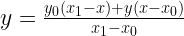
A bit of background before getting started. Linear interpolation is simply finding a value along a line between 2 known points. For given points (x₀ , y₀) and (x₁, y₁) the value at y for a known x can be calculated by the following

Since python is utilised, it is good practice to reuse existing functions already written by the community. It keeps your code clean, short, tidy and less prone to errors. Some of Python’s more common packages will be taken to task are NumPy and SciPy. These are described on their sites as:

NumPy is the fundamental package for scientific computing with Python. It contains among other things:

• a powerful N-dimensional array object
• sophisticated (broadcasting) functions
• tools for integrating C/C++ and Fortran code
• useful linear algebra, Fourier transform, and random number capabilities

SciPy (pronounced “Sigh Pie”) is open-source software for mathematics, science, and engineering.

To access the power of these packages is to just import them!

# import basic libraries
import numpy as np
from scipy import interpolate

Perusing through SciPy’s documentation, they have a tutorial specifically for Interpolation (how convenient). Right at the start is 1-D interpolation (interp1d) which looks like a good candidate.

The anatomy of the class is shown below. While simply using just x and y will work, I will be using some of the other parameters. Feel free to read the documentation details here

class scipy.interpolate.interp1d(x, y, kind=’linear’, axis=-1, copy=True, bounds_error=None, fill_value=nan, assume_sorted=False)[source]

I will elaborate a little on assume_sorted=False, bounds_error and fill_value .

assume_sorted is set to False by default, which means that the input data range for x can be in ascending or descending order. This greatly improves scalability as you don’t have to worry about the order. Originally I used numpy.interp but it only works with increasing values of x.

bounds_error is set to None by default, which will raise an error when interpolation is attempted on a value that is outside the range of x, either at the start (left side) or at the end (right side) of the x range. Personally, I don’t want to raise any errors in my code, therefore I will set it to False and deal with it in the fill values.

fill_value is set to nan (not a number) by default. In this example, I have specific requirements at both ends of the x range. Temperatures lower (or left of the range) have to be set at the allowable stress at the first input range of y. At the right side or end of the x range, temperatures higher (or right of the range) are not permitted, so I will set the allowable stress to 0.

# Interpolate a 1-D function using SciPy interpolate function

y_bound_xmin = y[0] # <-- First position in python starts at zero
y_bound_xmax = 0 # <-- right side set to zero stress

f = interpolate.interp1d(x, y, bounds_error=False, 
                                     fill_value=(y_bound_xmin, y_bound_xmax) )

After running the interpolate function, any value(s) of x has to be passed into f as either a single number or as many you like.

# find the interpolated results for the given x input(s)
f([30, design_temp, 601])

array([138.  ,  39.68,   0.  ])

Here I passed in the design temperature as well as both left and right out of bounds cases to show that the result was as expected.

To get a closer look at the design temperature conditions, a plot zoomed in on the area can be easily created within python.

4 Results

As I used this post in an engineering context, I will finish up with a calculation based on my linear interpreted value.

The equation used is in ASME B31.3-2018 Process Piping section 345.4.2 Test Pressure.

where
P = internal design gage pressure, MPa
P_T = minimum test gage pressure, MPa
S = allowable stress at component design temperature for the prevalent pipe material; see
Table A-1 or Table A-1M, MPa
S_T = allowable stress at test temperature for the prevalent pipe material; see Table A-1 or Table A-1M, MPa

b31_3_allow = f(design_temp)
stress_ratio = f(test_temp) / f(design_temp)
test_pres = 1.5 * design_pres * stress_ratio
test_ratio = test_pres / design_pres

Allowable Stress at test temperature: 138.0 MPa
Allowable Stress at design temperature: 38.1 MPa
Test Pressure: 100.0 MPa. Overall ratio to Design pressure: 5.4

Summary

Linear Interpolation using Python was performed using SciPy built-in interp1d function which easily caters for out of bound conditions. Compared to using Microsoft Excel which I covered previously, this is much for elegant and simpler.

I have included the full code on my Github page.

Disclaimer: I am a newbie to Python and am learning, therefore I’m sure my code may not be completely pythonic. If you have any comments or suggestions, please feel free to drop a comment below or hit me up on one of the socials.